A framework for simulation and inversion in electromagnetics
1Introduction
The field of electromagnetic (EM) geophysics encompasses a diverse suite of problems with applications across mineral and resource exploration, environmental studies and geotechnical engineering. EM problems can be formulated in the time or frequency domain. Sources can be grounded electric sources or inductive loops driven by time-harmonic or transient currents, or natural, plane wave sources, as in the case of the magnetotelluric method. The physical properties of relevance include electrical conductivity, magnetic permeability, and electric permittivity. These may be isotropic, anisotropic, and also frequency dependent. Working with electromagnetic data to discern information about subsurface physical properties requires that we have numerical tools for carrying out forward simulations and inversions that are capable of handling each of these permutations.
The goal of the forward simulation is to solve a specific set of Maxwell’s equations and obtain a prediction the EM responses. Numerical simulations using a staggered grid discretization Yee, 1966, have been extensively studied in their application for finite difference, finite volume and finite element approaches (c.f. Newman & Alumbaugh (1999)Haber (2014)), with many such implementations being optimized for efficient computations for the context in which they are being applied Haber & Ascher, 2001Li & Key, 2007Kelbert et al., 2014Yang et al., 2014.
Finding a model of the earth that is consistent with the observed data and prior geologic knowledge is the ‘inverse problem’. It presupposes that we have a means of solving the forward problem. The inverse problem is generally solved by minimizing an objective function that consists of a data misfit and regularization, with a trade-off parameter controlling their relative contributions. Tikhonov & Arsenin, 1977Parker, 1980Constable et al., 1987. Deterministic, gradient-based approaches to the inverse problem are commonplace in EM inversions. Relevance of the recovered inversion model is increased by incorporating a priori geologic information and assumptions. This can be accomplished through, the regularization term Oldenburg & Li, 2005Constable et al., 1987 or parameterizing the inversion model Pidlisecky et al., 2011McMillan et al., 2015Kang et al., 2015. Multiple data sets may be considered through cooperative or joint inversions Haber & Oldenburg, 1998McMillan et al., 2015.
Each of these advances relies on a workflow and associated software implementation. Unfortunately, each software implementation is typically developed as a stand-alone solution. As a result, these advances are not readily interoperable with regard to concepts, terminology, notations and software.
The advancement of EM geophysical techniques and the expansion of their application requires a flexible set of concepts and tools that are organized in a framework so that researchers can more readily experiment with, and explore, new ideas. For example, if we consider research questions within the growing application of EM for reservoir characterization and monitoring in settings with steel cased wells (cf. Hoversten et al. (2015)Um et al. (2015)Commer et al. (2015)Cuevas (2014)Hoversten et al. (2014)Pardo & Torres-Verdin (2013)), the numerical tools employed must enable investigation into factors such as the impact of variable magnetic permeability Wu & Habashy, 1994Heagy et al., 2015 and casing integrity brill2012 on electromagnetic signals. Various modelling approaches in both time and frequency domain simulations are being explored, these include employing highly-refined meshes Commer et al., 2015, using cylindrical symmetry Heagy et al., 2015 or approximating the casing on a coarse-scale Um et al., 2015, possibly 3D anisotropic approximations Caudillo-Mata et al., 2014. Beyond forward simulations that predict EM responses, to enable the interpretation of field data with these tools requires that machinery to address the inverse problem and experiment with approaches for constrained and/or time lapse inversions be in place Devriese & Oldenburg, 2016Marsala et al., 2015. Typically, addressing each of these complexities would require a custom implementations, particularly for the frequency domain and time domain simulations, although aspects, such as physical properties, are common to both. Inconsistencies between implementations and the need to implement a custom solution for each type of EM method under consideration presents a significant barrier to a researcher’s ability to experiment with and extend ideas.
Building from the body of work on EM geophysical simulations and inversions, the aim of our efforts is to identify a common, modular framework suitable across the suite of electromagnetic problems. This conceptual organization has been tested and developed through a numerical implementation. The implementation is modular in design with the expressed goal of affording researchers the ability to rapidly adjust, interchange, and extend elements. By developing the software in the open, we also aim to promote an open dialog on approaches for solving forward and inverse problems in EM geophysics.
The implementation we describe for EM forward and inverse problems extends a general framework for geophysical simulation and gradient based inverse problems, called SimPEG Cockett et al., 2015. The implementation of SimPEG is open-source, written in Python and has dependencies on the standard numerical computing packages NumPy, SciPy, and Matplotlib Walt et al., 2011Oliphant, 2007Hunter, 2007. The contribution described in this paper is the implementation of the physics engine for problems in electromagnetics, including the forward simulation and calculation of the sensitivities. Building within the SimPEG ecosystem has expedited the development process and allowed developments to be made in tandem with other applications (http://simpeg.xyz). simpegEM aspires to follow best practices in terms of documentation, testing, continuous integration using the publically available services Sphinx, Travis CI, and Coveralls Brandl, 2010Kalderimis & Meyer, 2011Merwin et al., 2015. As of the writing of this paper, when any line of code is changed in the open source repository, over 3 hours of testing is completed; documentation and examples are also tested and automatically updated (http://docs.simpeg.xyz). We hope these practices encourage the growth of a community and collaborative, reproducible software development in the field of EM geophysics.
The paper is organized as follows. To provide context for the structure and implementation of simpegEM, we begin with a brief overview of the SimPEG inversion framework as well as the governing equations for electromagnetics in Section 2. In Section 3, we discuss the motivating factors for the EM framework, and in Section 4, we discuss the framework and implementation of the forward simulation and calculation of sensitivities in simpegEM. We demonstrate the implementation with two synthetic examples and one field example in Section 5. The first example shows the similarities between the time and frequency implementations for a 1D inversion. In the second example, we invert field data from the Bookpurnong Irrigation district in Australia. The final example demonstrates how the modular implementation is used to compute the sensitivity for a parametric model of a block in a layered space where a transmitter is positioned inside a steel cased well.
2Background
We are focused on geophysical inverse problems in electromagnetics (EM), that is, given EM data, we want to find a model of the earth that explains those data and satisfies prior assumptions about the geologic setting. We follow the SimPEG framework, shown in Figure 1, which takes a gradient- based approach to the inverse problem Cockett et al., 2015. Inputs to the inversion are the data and associated uncertainties, a description of the governing equations, as well as prior knowledge and assumptions about the model. With these defined, the SimPEG framework accomplishes two main objectives:
the ability to forward simulate data and compute sensitivities (Forward Simulation - outlined in green in Figure 1),
the ability to assess and update the model in an inversion (Inversion Elements and Inversion as Optimization - outlined in red in Figure 1).
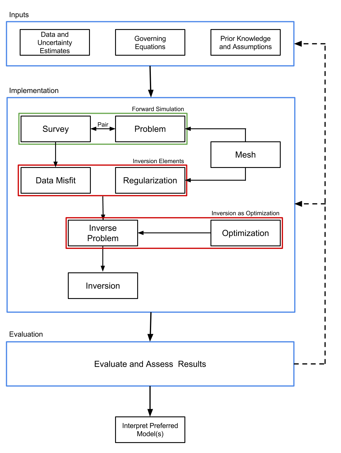
Figure 1:Inversion approach using the SimPEG framework. Adapted from Cockett et al. (2015)
The implementation of the framework is organized into the self-contained modules shown in Figure 1; each module is defined as a base- class within SimPEG. The Mesh provides the discretization and numerical operators. These are leveraged by the Problem, which is the numerical physics engine; the Problem computes fields and fluxes when provided a model and Sources. The Sources are specified in the Survey, as are the Receivers. The Receivers take the Fields computed by the Problem and evaluate them at the receiver locations to create predicted data. Each action taken to compute data, when provided a model, has an associated derivative with respect to the model; these components are assembled to create the sensitivity. Having the ability to compute both predicted data and sensitivities accomplishes the first objective.
To accomplish the second objective of assessing and updating the model in the context of the data and our assumptions, we consider a gradient-based approach to the inversion. For this, we specify an objective function which generally consists of a DataMisfit and Regularization. The DataMisfit is a metric that evaluates the agreement between the observed and predicted data, while the Regularization is a metric constructed to assess the model’s agreement with assumptions and prior knowledge. These are combined with a trade-off parameter to form a mathematical statement of the InvProblem, an optimization problem. The machinery to update the model is provided by the Optimization. An Inversion brings all of the elements together and dispatches Directives for solving the InvProblem. These Directives are instructions that capture the heuristics for solving the inverse problem; for example, specifying a target misfit that, once reached, terminates the inversion, or using a beta-cooling schedule that updates the value of the trade-off parameter between the DataMisfit and Regularization (cf. Parker (1994)Oldenburg & Li (2005) and references within).
The output of this process is a model that must be assessed and evaluated prior to interpretation; the entire process requires iteration by a human, where underlying assumptions and parameter choices are re-evaluated and challenged. Be it in resource exploration, characterization or development; environmental remediation or monitoring; or geotechnical applications – the goal of this model is to aid and inform a complex decision.
Here we note that the inversion framework described above is agnostic to the type of forward simulation employed, provided the machinery to solve the forward simulation and compute sensitivities is implemented. Specific to the EM problem, we require this machinery for Maxwell’s equations. As such, we focus our attention on the Forward Simulation portion of the implementation for the EM problem and refer the reader to Cockett et al. (2015) and Oldenburg & Li (2005) for a more complete discussion of inversions.
2.1Governing Equations
Maxwell’s equations are the governing equations of electromagnetic problems. They are a set of coupled partial differential equations that connect electric and magnetic fields and fluxes. We consider the quasi-static regime, ignoring the contribution of displacement current Ward & Hohmann, 1988Telford et al., 1990Haber, 2014 [1]
We begin by considering the first order quasi-static EM problem in time,
where , are the electric and magnetic fields, is the magnetic flux density, is the current density, and , are the magnetic and electric source terms. is a physical, electric current density, while is “magnetic current density”. Although is unphysical, as continuity of the magnetic current density would require magnetic monopoles, the definition of a magnetic source term can be a useful construct, as we will later demonstrate in Section 4 (see also Ward & Hohmann (1988)).
By applying the Fourier Transform (using the convention), we can write Maxwell’s equations in the frequency domain:
where we use capital letters to denote frequency domain variables. The fields and fluxes are related through the physical properties: electrical conductivity σ, and magnetic permeability μ, as described by the constitutive relations
The physical properties, σ and μ are generally distributed and heterogeneous. For isotropic materials, σ and μ are scalars, while for anisotropic materials they are symmetric positive definite tensors. The same constitutive relations can be applied in the time domain provided that the physical properties, σ, μ are not frequency-dependent.
In an EM geophysical survey, the sources provide the input energy to excite responses that depend on the physical property distribution in the earth. These responses, electric and magnetic fields and fluxes, are sampled by receivers to give the observed data. The simulation of Maxwell’s equations may be conducted in either the time or frequency domain, depending on the nature of the source; harmonic waveforms are naturally represented in the frequency domain, while transient waveforms are better described in the time domain.
The aim of the inverse problem is to find a model, (which may be a voxel-based or a parametric representation) that is consistent with observed data and with prior knowledge and assumptions about the model. Addressing the inverse problem using a gradient-based approach requires two abilities of the forward simulation: (1) the ability to compute predicted data given a model
and (2) the ability to compute or access the sensitivity, given by
To employ second order optimization techniques, we also require the adjoint of the sensitivity, . These two elements, when combined into the SimPEG framework, enable data to be simulated and gradient-based inversions to be run. As such, this work benefits from other peoples’ contributions to the underlying inversion machinery, including: discrete operators on a variety of meshes, model parameterizations, regularizations, optimizations, and inversion directives Cockett et al., 2015.
3Motivation
The motivation for the development of this framework is that it be a resource for researchers in the field of electromagnetic geophysics. To best serve this goal, we require a framework that is modular and extensible in order to enable exploration of ideas. An associated numerical implementation is essential for this work to be tested and acted upon. As such, we provide a tested, documented, fully open-source software implementation of the framework (under the permissive MIT license).
Specific to the EM problem, we require the implementation of Maxwell’s equations in both the time domain and frequency domain. The implementation must allow for variable electrical conductivity and magnetic permeability, anisotropic physical properties; various model parameterizations of the physical properties (e.g. voxel log-conductivity or parametric representations); a range of sources including wires, dipoles, natural sources; variable receiver types; variable formulations of Maxwell’s equations; solution approaches such as using a primary-secondary formulation; and the flexibility to work with and move between a variety of meshes such as tensor, cylindrically symmetric, curvilinear, and octree discretizations. Furthermore, the sensitivity computation must be flexible enough to be computed for any sensible combination of these approaches. In the following section, we will outline the framework we have used to organize and implement these ideas.
4Simulation Framework
The aim of the forward simulation is to compute predicted data, , when provided with an inversion model[2], and Sources. simpegEM contains implementations for both time domain (TDEM) and frequency domain (FDEM) simulations, allowing data from commonly used EM methods to be simulated.
The framework we follow to perform the forward simulation is shown in Figure 2; it consists of two overarching categories:
the
Problem, which is the implementation of the governing equations,the
Survey, which provides the source(s) to excite the system as well as the receivers to samples the fields and produce predicted data at receiver locations.
Here, we provide a brief overview of each of the components, and discuss them in more detail in the sections that follow.
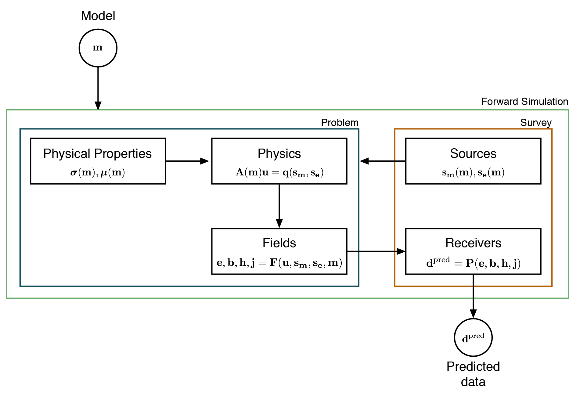
Figure 2:Forward simulation framework.
The ‘engine’ of the forward simulation is the physics; it contains the machinery to solve the system of equations for EM fields and fluxes in the simulation domain when provided with a description of the physical properties and sources. In general, the physics engine may be an analytic or numeric implementation of Maxwell’s equations. Here, we focus our attention on the numerical implementation using a standard staggered-grid finite volume approach, requiring that the physical properties, fields, fluxes and sources be defined on a mesh (cf. Haber (2014)Hyman et al. (2002)Hyman & Shashkov (1999)Yee (1966)). We discretize fields on edges, fluxes on faces and physical properties in cell centers, as shown in Figure 3. To construct the necessary differential and averaging operators, we leverage the Mesh class within SimPEG Cockett et al., 2015Cockett et al., 2016.
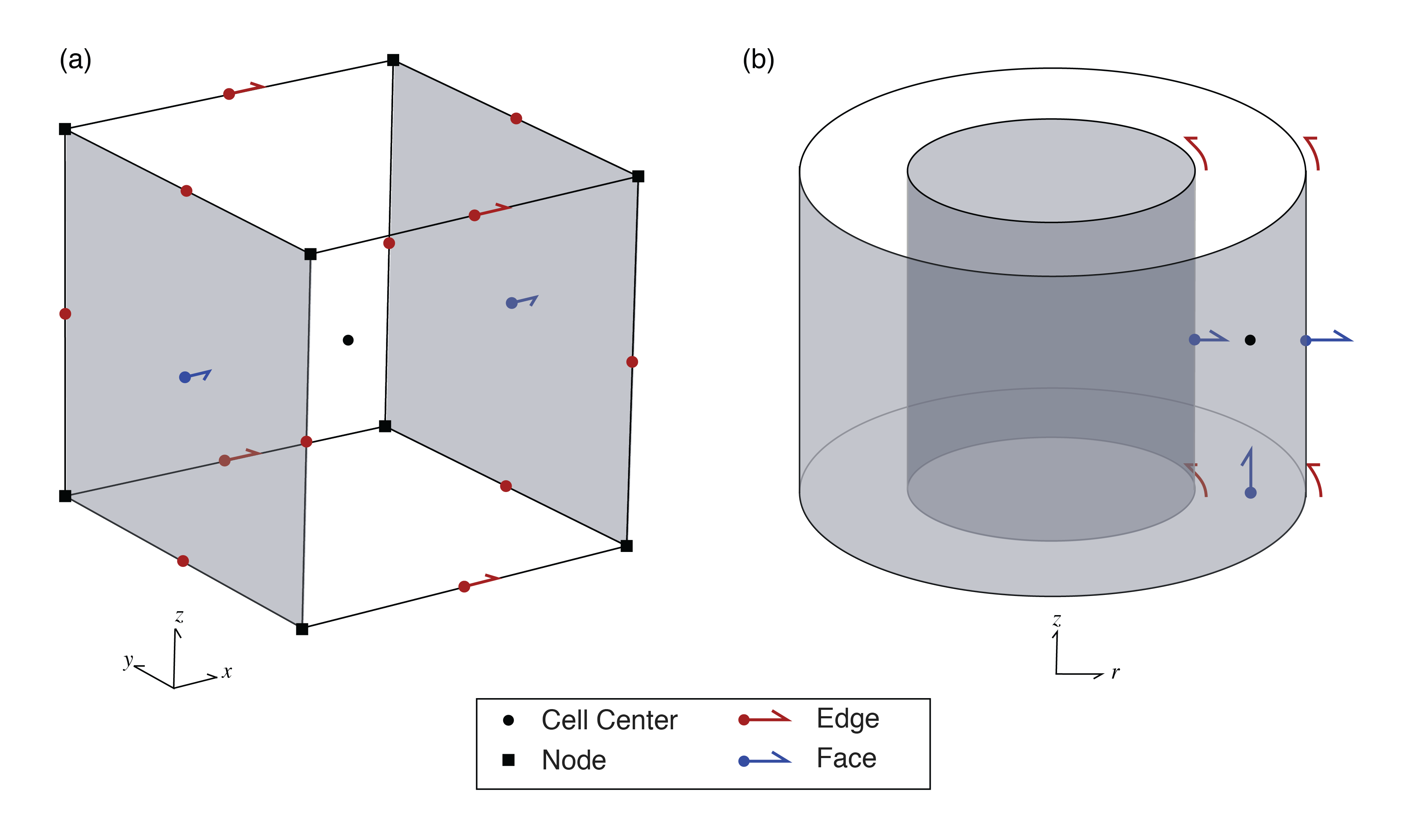
Figure 3:Location of variables in the finite volume implementation for both a unit cell in (a) cartesian and (b) cylindrical coordinates (after Heagy et al. (2015))
To compute electromagnetic responses, the forward simulation requires the definition of a physical property model describing the electrical conductivity () and magnetic permeability () on the simulation mesh, as well as discrete representations of the sources used to excite EM responses (. Often in solving an inverse problem, the model which one inverts for (the vector ), is some discrete representation of the earth that is decoupled from the physical property model. This decoupling requires the definition of a Mapping capable of translating to physical properties on the simulation mesh. For instance, if the inversion model is chosen to be log-conductivity, an exponential mapping is required to obtain electrical conductivity (i.e. )). To support this abstraction, SimPEG provides a number of extensible Mapping classes Cockett et al., 2015Kang et al., 2015.
With both the physical property model and the source specified, we define and solve the physics, a Maxwell system of the form
for an electric or magnetic field or flux. Here, is the system matrix that may eliminate a field or flux to obtain a system in a single field or flux, , the solution vector. Correspondingly, the vector is the second order right-hand-side. Note, if there are necessary manipulations to make equation 6 easier to solve numerically (e.g. symmetry) we can add these here; doing so has no effect on the derivative. The remaining fields and fluxes can be computed from anywhere in the simulation domain, through an operation of the form
where is conceptually a vector of all of the fields and fluxes (i.e. , , and ). This vector is never stored in the implementation, instead the fields are computed on demand through the subset of stored solution vectors (). From the computed fields (), predicted data are created by the Receivers through an operation of the form
In the simplest case, the action of selects the component of interest and interpolates the fields to the receiver locations, more involved cases could include the computation of ratios of fields, as is the case for impedance or tipper data. Obtaining predicted data from the framework concludes the forward simulation.
The same framework is employed for both time domain (TDEM) and frequency domain (FDEM) implementations within simpegEM. In the case of the FDEM implementation, the matrix and the solution vector represent all frequencies. As these frequencies are independent (i.e. a block diagonal matrix,

), each frequency can be solved independently. In the TDEM code, the matrix and the solution vector represent all timesteps Oldenburg et al., 2013Haber, 2014 and take the form of a lower triangular block matrix (bidiagonal in the case of Backward Euler,

), meaning the computation of each time-step depends on previous time-steps. The form of these matrices will be discussed further in the Physics section (Section 4.2)
To perform a gradient-based inversion, we require the sensitivity of the data with respect to the inversion model, thus, each action taken to calculate data from the model must have an associated derivative. The full sensitivity is a dense matrix and is expensive to form and store, but when the optimization problem is solved using an iterative optimization approach, it does not need to be explicitly formed; all that is required are products and adjoint-products with a vector. We treat this using a modular approach so that individual elements of the framework can be rapidly interchanged or extended. The process we follow to compute matrix-vector products with the sensitivity is shown with red arrows in Figure 4 (b). The sensitivity-vector product is built in stages by taking matrix vector products with the relevant derivatives in each module, starting with the derivative of the physical property with respect to the model. The product with the adjoint is similarly shown in Figure 4 (c) starting with the adjoint of the receiver operation.
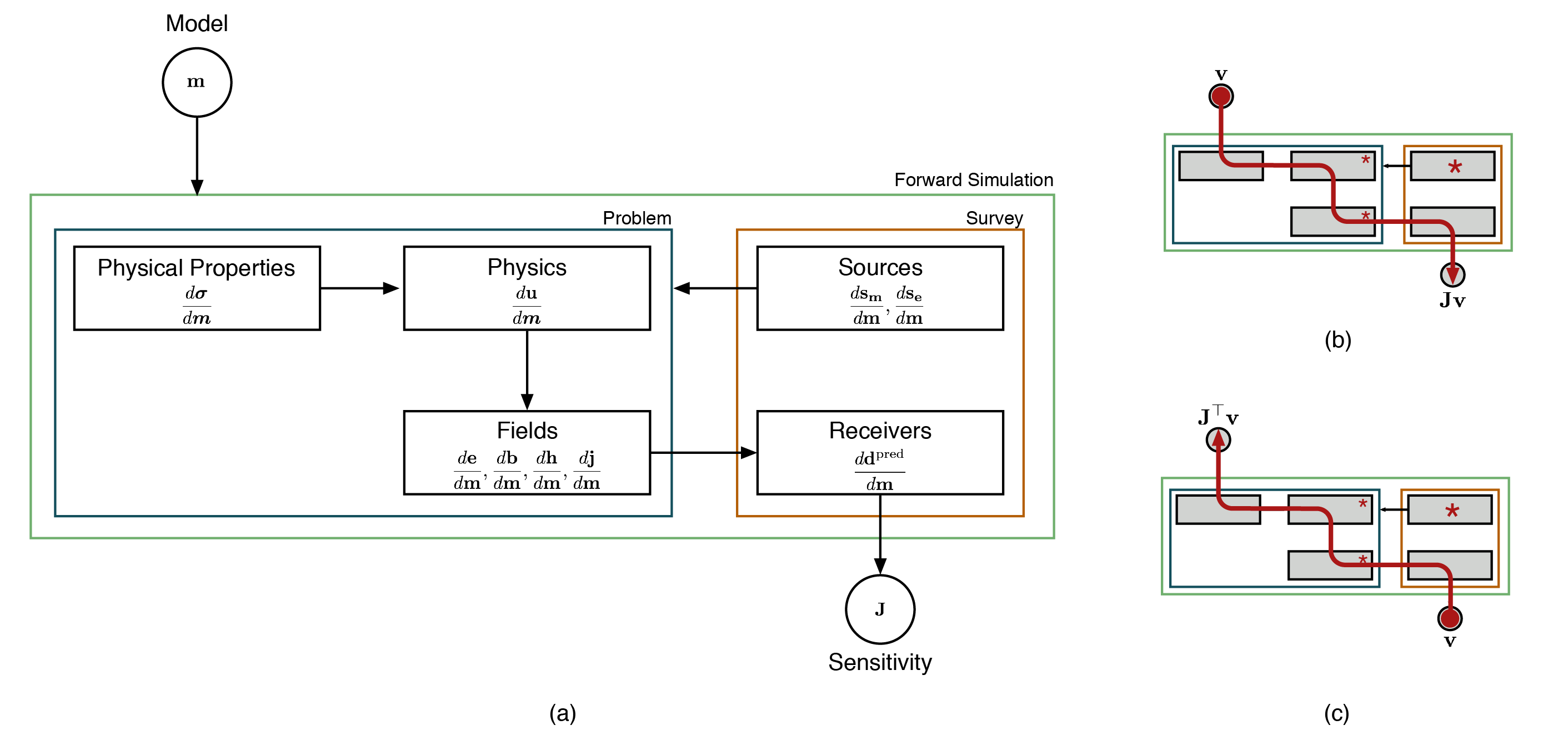
Figure 4:(a) Contributions of each module to the sensitivity. (b) process for computing and (c) ; stars indicate where the source derivatives are incorporated.
Using electrical conductivity, , as the only active property described by the inversion model for brevity, the sensitivity takes the form
The annotations denote which of the elements shown in Figure 4 are responsible for computing the respective contribution to the sensitivity. If the model provided is in terms of or a source/receiver location, this property replaces the role of . The flexibility to invoke distinct properties of interest (e.g. σ, μ, source location, etc.) in the inversion requires quite a bit of ‘wiring’ to keep track of which model parameters are associated with which properties; this is achieved through a property mapping or PropMap (physical properties, location properties, etc.) within SimPEG.
Although typically the source terms do not have model dependence and thus their derivatives are zero, the derivatives of and must be considered in a general implementation. For example, if one wishes to use a primary-secondary approach, where source fields are constructed by solving a simplified problem, the source terms may have dependence on the model meaning their derivatives have a non-zero contribution to the sensitivity (c.f. Coggon1971Haber (2014)Heagy et al. (2015)); this will be demonstrated in the Casing Example in Section 5.3.
The derivative of the solution vector with respect to the model is found by implicitly taking the derivative of equation 6 with respect to , giving
The annotations below the equation indicate the methods of the Problem class that are responsible for calculating the respective derivatives. Typically the model dependence of the system matrix is through the physical properties (i.e. σ, μ). Thus, to compute derivatives with respect to , the derivatives are first taken with respect to and the dependence of on is treated using chain rule. The chain rule dependence is computed and tested automatically in SimPEG using the composable Mapping classes.
In the following sections, we discuss the implementation of elements shown in Figure 2 and highlight their contribution to the forward simulation and calculation of the sensitivity. We begin by discussing the inversion model and its relationship to the physical properties (Section 4.1), move on to the core of the forward simulation, the Physics (Section 4.2), and to how Sources which excite the system are defined (Section 4.3). Following these, we then discuss how Fields are calculated everywhere in the domain (Section 4.4) and how they are evaluated by the Receivers to create predicted data (Section 4.5). We conclude this section with a Summary and discussion on testing (Section 4.6).
4.1Model and Physical Properties
For all EM problems, we require an inversion model that can be mapped to meaningful physical properties in the discretized Maxwell system. Typically, we consider the model to be a description of the electrical conductivity distribution in the earth. Often, the model is taken to be log-conductivity, in which case, an exponential mapping is required (ExpMap) to convert the model to electrical conductivity. The inversion model may be defined on a subset of a mesh and referred to as an ‘active cell’ model. For instance, air cells may be excluded and only the subsurface considered; in this case an InjectActiveCells map is used to inject the active model into the full simulation domain. In the case of a parametric inversion, the inversion model is defined on a domain that is independent of the forward modelling mesh and the mapping takes the parametric representation and defines a physical property on the forward modelling mesh (e.g. a gaussian ellipsoid defined geometrically) MaokunLi2010Pidlisecky et al., 2011McMillan et al., 2015Kang et al., 2015. Maps can be composed, for instance, a layered, 1D log conductivity model defined only in the subsurface may be mapped to a 2D cylindrical Mesh, as shown in Figure 5.
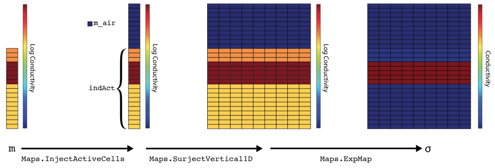
Figure 5:Mapping an inversion model, a 1D layered, log conductivity model defined below the surface, to electrical conductivity defined in the full simulation domain.
    import numpy as np
    from SimPEG import Mesh, Maps
    mesh = Mesh.CylMesh([20, 20])    # SimPEG cylindrically symmetric mesh
    m_air = np.log(1e-8)             # value of the model in the air cells
    indAct = mesh.vectorCCz < 0.0    # define active cells to be subsurface only
    mapping = ( Maps.ExpMap(mesh) *
                Maps.SurjectVertical1D(mesh) *
                Maps.InjectActiveCells(mesh, indAct, m_air, nC=mesh.nCz) )
In the code above, the ‘multiplication’ performs the composition of the mappings. For the contribution of this action to the sensitivity, the derivative of the electrical conductivity with respect to the model is computed using the chain rule for the composed maps (cf. Kang et al. (2015)Heagy et al. (2014)). During an inversion, the electrical conductivity on the simulation mesh associated with the current inversion model and its derivative are accessed through the BaseEMProblem, which is inherited by both the TDEM and FDEM problems. In some cases, variable magnetic permeability must be considered; this is accomplished through a property mapping (PropMap). The PropMap handles the organization and independent mappings of distinct physical properties (i.e. , ).
4.2Physics
To formulate a system of equations from Maxwell’s equations in time (equation 1) or frequency (equation 2) that can be solved numerically using a finite volume approach, we require a statement of the problem in terms of two equations with two unknowns, one of which is a field (discretized on edges), and the other a flux (discretized on faces). Thus, we can consider either the E-B formulation, or the H-J formulation. For the frequency-domain problem, we can discretize the electric field, , on edges, the magnetic flux, , on faces, physical properties σ and at cell centers, and the source terms and on faces and edges, respectively (see Figure 3). Doing so, we obtain the discrete system:
where is the discrete edge curl, is the face inner-product matrix for , is the edge inner-product matrix for ; these inner product matrices can be computed for isotropic, diagonally anisotropic or fully anisotropic physical properties using operators within SimPEG’s Mesh class Cockett et al., 2015Cockett et al., 2016.
Note that the source-term is an integrated quantity. Alternatively, the H-J formulation discretizes on edges, on faces, ρ and μ at cell centers, and the source terms , on edges and faces, respectively, giving
Similarly, is an integrated quantity. In a full 3D simulation, the electric and magnetic contributions for the two formulations are merely staggered from one another. However, if using an assumption of cylindrically symmetry, the appropriate formulation must be used to simulate either rotational electric or magnetic contributions Heagy et al., 2015. For both the basic FDEM and TDEM implementations, natural boundary conditions ( in E-B formulation or in H-J formulation), in which the fields are assumed to have decayed to a negligible value at the boundary, are employed to construct the differential operators, the framework and implementation are however, extensible to consider other boundary conditions (cf. Haber (2014)Rivera Rios (2014)).
In order to solve either equation 11 or equation 12, we eliminate one variable and solve the second order system. This elimination is performed by the FDEM problem classes. For instance, in FDEM Problem_e, we eliminate and obtain a second order system in
FDEM Problem_e has methods getA and getRHS to construct the system and associated methods getADeriv and getRHSDeriv to construct the derivatives of each with respect to the inversion model. These function definitions are methods of the Problem class, where the self variable refers to the instance of the class, and is standard Python (cf. Python documentation - https://docs.python.org/3/tutorial/classes.html). For FDEM Problem_e, getRHSDeriv is zero unless one or both of the source terms have model dependence. However, if we eliminate and solve for (Problem_b), the right hand side contains the matrix , and therefore will, in general, have a non-zero derivative. To solve this linear system of equations, SimPEG interfaces to standard numerical solver packages (e.g. SciPy, Mumps Oliphant, 2007Amestoy et al., 2001Amestoy et al., 2006, using for example pymatsolver https://github.com/rowanc1/pymatsolver). The components used to perform the forward simulation are assembled in the fields method of the BaseFDEMProblem class; the fields method solves the forward simulation for the solution vector (from equation 13) at each frequency and source considered.
Similarly, for the time-domain problem, the semi-discretized E-B formulation is given by
and the semi-discretized H-J formulation is given by
For the time discretization, we use Backward Euler (cf. Ascher (2008)). To form the TDEM Problem_b, we eliminate from equation 14 and apply Backward Euler for the time discretization. A single timestep takes the form
where is the timestep and the superscripts , indicate the time index. Each TDEM problem formulation (ie. Problem_e, Problem_b, Problem_h, Problem_j) has methods to create the matrices along the block-diagonals,
and , as well as a method to construct the right hand side, , at each timestep. When inverting for a model in electrical conductivity using Problem_b, the subdiagonal matrices are independent of , however, in other formulations, such as Problem_e, the subdiagonal matrices do have dependence on electrical conductivity, thus in general, the model dependence must be considered. Depending on the solver chosen, it can be advantageous to make the system symmetric; this is accomplished by multiplying both sides by . To solve the full time-stepping problem, we assemble all timesteps in a lower block bidiagonal matrix, with on-diagonal matrices and sub-diagonal matrices , giving
When solving the forward simulation, the full time-stepping matrix, , is not formed, instead the block system is solved using forward substitution with each block-row being computed when necessary. The initial condition, , depends on the source type and waveform; it is computed numerically or specified using an analytic solution. For example, if using a grounded source and a step-off waveform, is found by solving the direct current resistivity or the magnetometric resistivity problem, depending on which field we choose to solve for. When a general current waveform is considered, the initial condition will be , and either or , depending on type of the source used, will have non-zero values during the on-time.
Derivatives of the matrices along the block-diagonals of along with derivatives of the right-hand-side are stitched together in a forward time stepping approach to compute the contribution of to and in a backwards time stepping approach for the contribution of to .
4.3Sources
Sources input EM energy into the system. They can include grounded wires, loops, dipoles and natural sources. Controlled sources are implemented in the FDEM and TDEM modules of simpegEM, and natural sources are implemented in the NSEM module. For simulations, we require that the sources be discretized onto the mesh so that a right-hand-side for the Maxwell system can be constructed (i.e. getRHS). This is addressed by the eval method of the source which returns both the magnetic and electric sources (, shown in Figure 2) on the simulation mesh.
In some cases, a primary-secondary approach can be advantageous for addressing the forward problem (cf. Coggon1971Haber (2014)Heagy et al. (2015)). We split up the fields and fluxes into primary and secondary components (, ) and define a “Primary Problem”, a simple problem, often with an analytic solution, that is solved in order to construct a source term for a secondary problem. For instance, a point magnetic dipole source may be simulated by defining a zero-frequency primary which satisfies
If we define to be a constant, equation 18 has an analytic solution for that may be expressed in terms of a curl of a vector potential (cf. Griffiths (2007)). When using a mimetic discretization, by defining the vector potential and taking a discrete curl, we maintain that the magnetic flux density is divergence free as the divergence operator is in the null space of the edge curl operator (), so numerically we avoid creating magnetic monopoles (c.f. Haber (2014)). The secondary problem is then
The source terms for the secondary problem are and . In scenarios where magnetic permeability is homogeneous, the electric source contribution is zero.
The left hand side is the same discrete Maxwell system as in equation 11; the distinction is that we are solving for secondary fields, and a primary problem was solved (analytically or numerically) in order to construct the source terms. To obtain the total fields, which we sample with the receivers, we must add the primary fields back to the solution. To keep track of the primary fields, they are assigned as properties of the source class.
In most cases, source terms do not have a derivative with respect to the model. However, in a primary-secondary problem in electrical conductivity the source term depends on the electrical conductivity and derivatives must be considered (see Section 5.3). This is similar to inverting for magnetic permeability using a primary-secondary approach described in equation 19 Coggon1971Haber, 2014Heagy et al., 2015. It is also possible to consider your inversion model to be the location or waveform of the source, in which case the derivative is also non-zero and source derivatives can be included in the optimization procedure.
4.4Fields
By solving the second-order linear system, as in equation 13, we obtain a solution vector, , of one field or flux everywhere in the domain. In the case of a primary-secondary problem, this solution is a secondary field. To examine all of the fields, we require easy access to the total fields and total fluxes everywhere in the domain. This is achieved through the Fields object.
For efficient memory usage, only the solution vector is stored, all other fields and fluxes are calculated on demand through matrix vector multiplications. As such, each problem type (e, b, h, j) has an associated Fields object with methods to take the solution vector and translate it to the desired field or flux. For instance, Fields_j stores the solution vector from Problem_j and has methods to compute the total magnetic field in the simulation domain by first computing the secondary magnetic field from the solution vector (; in this example, ) and adding back any contribution from the source
For their contribution to the sensitivity (equation 9), the fields have methods to compute derivatives when provided the vectors and (from the Physics). For instance, for
The derivatives for , , and take the same form. Conceptually, the product of the full derivative and a vector can be thought of as a stacked vector of all of the contributions from all of the fields and fluxes, however, this is never formed in practice.
4.5Receivers
The measured data consist of specific spatial components of the fields or fluxes sampled at the receiver locations at a certain time or frequency. Receivers have the method eval that interpolates the necessary components of the fields and fluxes to the receiver locations and evaluates the data required for the problem, such as the frequency domain fields or natural source impedance data. For the frequency domain problem, real and imaginary components are treated as separate data so that when inverting, we are always working with real values. The separation of the data evaluation from fields in receiver objects allows the derivative computation to be performed and tested in a modular fashion; this enables rapid development and implementation of new receiver types.
4.6Summary
Having defined the role of each of the elements in the forward simulation framework outlined in Figure 2, the necessary machinery to compute predicted data and sensitivities is at hand for both FDEM and TDEM problems. The modular nature of the framework allows us to make several abstractions which make the code more transparent and ensure consistency across implementations. For instance, the definition of the physical properties and associated inner product matrices is common to all formulations in both time and frequency domains. Thus, these are defined as properties of a BaseEM class which is inherited by both the TDEM and FDEM modules. Within each of the TDEM and FDEM modules, common methods for the calculation of the fields, sensitivities and adjoint are defined and shared across the approaches that solve for , , , or (see the documentation http://docs.simpeg.xyz).
Testing is conducted using comparisons with analytics, cross-comparisons between formulations, order tests on the sensitivity, adjoint tests, examples, tests on the finite volume operators, projections, interpolations, solvers, etc. Tests are run upon each update to the repository through the continuous integration service TravisCI Kalderimis & Meyer, 2011. This ensures that we can trust the tools that we use and move faster in our research into new methods and implementations. This also supports new developers and researchers in contributing to the code base without fear of breaking assumptions and ideas laid out by previous development.
5Examples
To demonstrate the application and structure of the framework, we explore three examples, one field example and two synthetic examples. The purpose of the first synthetic example is to show simple time and frequency domain electromagnetic inversions, and highlight the common framework. For this, we invert for a 1D layered Earth using a 2D cylindrically symmetric mesh for the forward simulation. In the second example, we show 1D inversions of field data (RESOLVE and SkyTEM) collected over the Bookpurnong Irrigation district in Australia. The final example is a 3D synthetic example that demonstrates a sensitivity analysis using a parametric model of a block in a layered space for a reservoir characterization problem where the transmitter is positioned down-hole in a steel-cased well. We use this example to demonstrate how mappings, multiple physical properties (both electrical conductivity and magnetic permeability), and multiple meshes, a cylindrically symmetric and a 3D tensor mesh, can be composed in a primary-secondary approach for performing the forward simulation and computing the sensitivities. The scripts used to run these examples are available on http://docs.simpeg.xyz.
5.1Cylindrically Symmetric Inversions
The purpose of this example is to demonstrate the implementation of the electromagnetic inversion in both time and frequency domains. We have chosen this example as it is computationally light, can be run on any modern laptop without installing complex dependencies, and yet it uses most of the elements and functionality needed to solve a large 3D EM problem. The script used to run this simulation is available at: https://doi.org/10.6084/m9.figshare.5035175.
We consider two 1D inversions for log-conductivity from an EM survey, one frequency domain experiment and one time domain experiment. Both surveys use a vertical magnetic dipole (VMD) source located on the surface. For simplicity, we consider a single receiver, measuring the vertical magnetic field, located 50m radially away from the source. The magnetic permeability is taken to be that of free space (), and electrical conductivity is assumed to be frequency-independent.
Figure 6 shows the setup used for: (a) the frequency domain simulation, (b) the time domain simulation, and (c) the common inversion implementation. In both, a cylindrical mesh is employed for the forward simulation and a 1D layered earth, described in terms of log-conductivity. To map the inversion model to electrical conductivity, a composite mapping is used to inject the 1D subsurface model into one including air cells (InjectActiveCells), surject the 1D model onto the 2D simulation mesh (SurjectVertical1D) and take the exponential to obtain electrical conductivity (ExpMap), as described in the Model and Physical Properties section (Section 4.1).
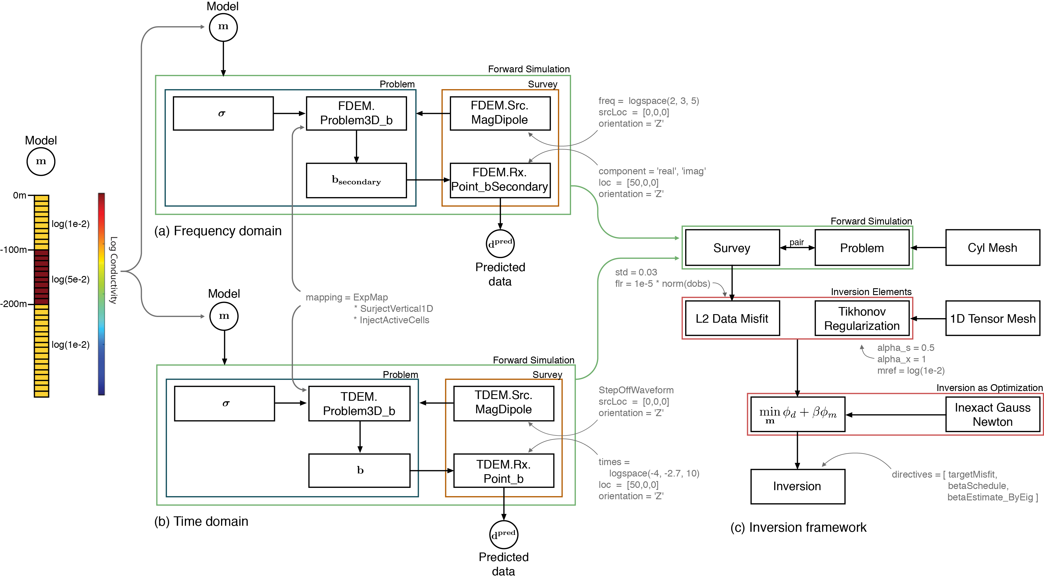
Figure 6:Diagram showing the entire setup and organization of (a) the frequency domain simulation; (b) the time domain simulation; and (c) the common inversion framework used for each example. The muted text shows the programmatic inputs to each class instance.
The distinction between the frequency and time domain inversions comes in the setup of the forward simulations. Each employs the appropriate description of the physics (FDEM or TDEM) in the problem, and the definition of the survey, consisting of both sources and receivers, must be tailored to the physics chosen. For the FDEM survey, a vertical harmonic magnetic dipole located at the origin transmits at five frequencies logarithmically spaced between 100 Hz and 1000 Hz. The receiver is located at (50 m, 0 m, 0 m) and measures the secondary magnetic flux (with the primary being the free-space response of a harmonic magnetic dipole). The observed response is complex- valued, having both real and imaginary components. We consider these as separate data, giving a total of ten data points for this example. For the time domain survey, we again use a vertical magnetic dipole at the origin, however, we now use a step-off waveform. The observed responses are defined through time, and thus are all real-valued. For this example, we sample 10 time channels, logarithmically spaced between and . These time channels were selected to be sensitive to depths similar to the FDEM simulation.
With the forward simulation parameters defined in both the time and frequency domain simulations, we can generate synthetic data. The model used consists of a 100m thick conductive layer (0.05 S/m) whose top boundary is 100 m-below from the surface, as shown in Figure 6. The conductivity of the half-space earth is 0.01 S/m. In both cases, 3% gaussian noise is added to the simulated data, and these are treated as the observed data () for the inversion.
For the inversions, we specify the inversion elements: a data misfit and a regularization. We use an L2 data misfit of the form
where and we define . For both simulations the floor is set to . The regularization is chosen to be a Tikhonov regularization on the 1D model
where is the reference model which is set to be a half- space of . The matrix is a 1D gradient operator. For both examples and . The data misfit and regularization are combined with a trade-off parameter, β, in the statement of the inverse problem. To optimize, we use the second-order Inexact Gauss Newton scheme. In this inversion, we use a beta-cooling approach, where β is reduced by a factor of 4 every 3 Gauss Newton iterations.
The initial β is chosen to relatively weight the influence of the data misfit and regularization terms. We do this by estimating the largest eigenvalue of and using one iteration of the power method. We then take their ratio and multiply by a scalar to weight their relative contributions. For this example, we used a factor of 10. For a stopping criteria, we use the discrepancy principle, stopping the inversion when , with and (with as defined in equation 22.)
The FDEM inversion reaches the target misfit after 9 iterations, and the TDEM inversion reaches the target misfit after 6 iterations. Figure 7 shows the recovered models (a), predicted and observed data for the FDEM inversion (b) and predicted and observed data for the TDEM inversion (c). In both the FDEM and TDEM inversions, the data are fit well. The recovered models are smooth, as is expected when employing an L2, Tikhonov regularization and both the location and amplitude of the conductive layer. The structure of both models are comparable, demonstrating that the information content in both the FDEM and TDEM data are similar. The recovered model can be improved by many additional techniques that are not explored here (e.g. using compact norms in the regularization). The SimPEG package provides a number of additional directives and regularization modules which can be useful for this purpose.

Figure 7:(a) True and recovered models for the FDEM and TDEM inversions; predicted and observed data for (b) the FDEM example, and (c) the TDEM example. In (b) the magnetic field data are in the negative z-direction.
5.2Bookpurnong Field Example
The purpose of this example is to demonstrate the use of the framework for inverting field data and provide an inversion that can be compared with other results in the literature. In particular, we invert frequency and time domain data collected over the Bookpurnong Irrigation District in Southern Australia. The Murray River and adjacent floodplain in the Bookpurnong region have become extensively salinized, resulting in vegetation die-back Munday et al., 2006Overton et al., 2004. Multiple electrical and electromagnetic data sets have been collected with the aim of characterizing the near-surface hydrologic model of the area Munday et al., 2006. For a more complete background on the geology and hydrogeology of the Bookpurnong region, we refer the reader to Munday et al. (2006).
Here, we will focus our attention to the RESOLVE frequency-domain data collected in 2008 and the SkyTEM time-domain data collected in 2006. These data are shown in Figure 8. The RESOLVE system consists of 5 pairs of horizontal coplanar coils, with nominal frequencies of 400 Hz, 1800 Hz, 8200 Hz, 40 000 Hz, and 130 000 Hz as well as a vertical coaxial coil pair of coils which operates at 3200Hz. For the Bookpurnong survey, the bird was flown at 50m altitude Viezzoli et al., 2010. The SkyTEM time-domain system operates in two transmitter modes that can be run sequentially. The high moment mode has high current and operates at a low base frequency (25 Hz and can be lowered to 12.5 Hz), and the low moment operates at a lower current and higher base frequency (222.5 Hz) Sørensen & Auken, 2004. The Bookpurnong SkyTEM survey was flown at an altitude of 60m Viezzoli et al., 2010.
Multiple authors have inverted these data sets; 1D spatially constrained inversions of the SkyTEM and RESOLVE data were performed by Viezzoli et al., 2009Viezzoli et al., 2010. Yang (2017) independently inverted these data in 1D and provides a discussion at http://em.geosci.xyz/content/case_histories/bookpurnong/index.html. The SkyTEM data (high moment) were inverted in 3D by Wilson et al., 2010. In the example that follows, we select a location where both the RESOLVE and SkyTEM datasets have soundings and invert them in 1D, we then proceed to perform a stitched 1D inversion of the RESOLVE data. The data have been made available with the permission of CSIRO and are accessible, along with the script used to run the inversions at https://doi.org/10.6084/m9.figshare.5107711.
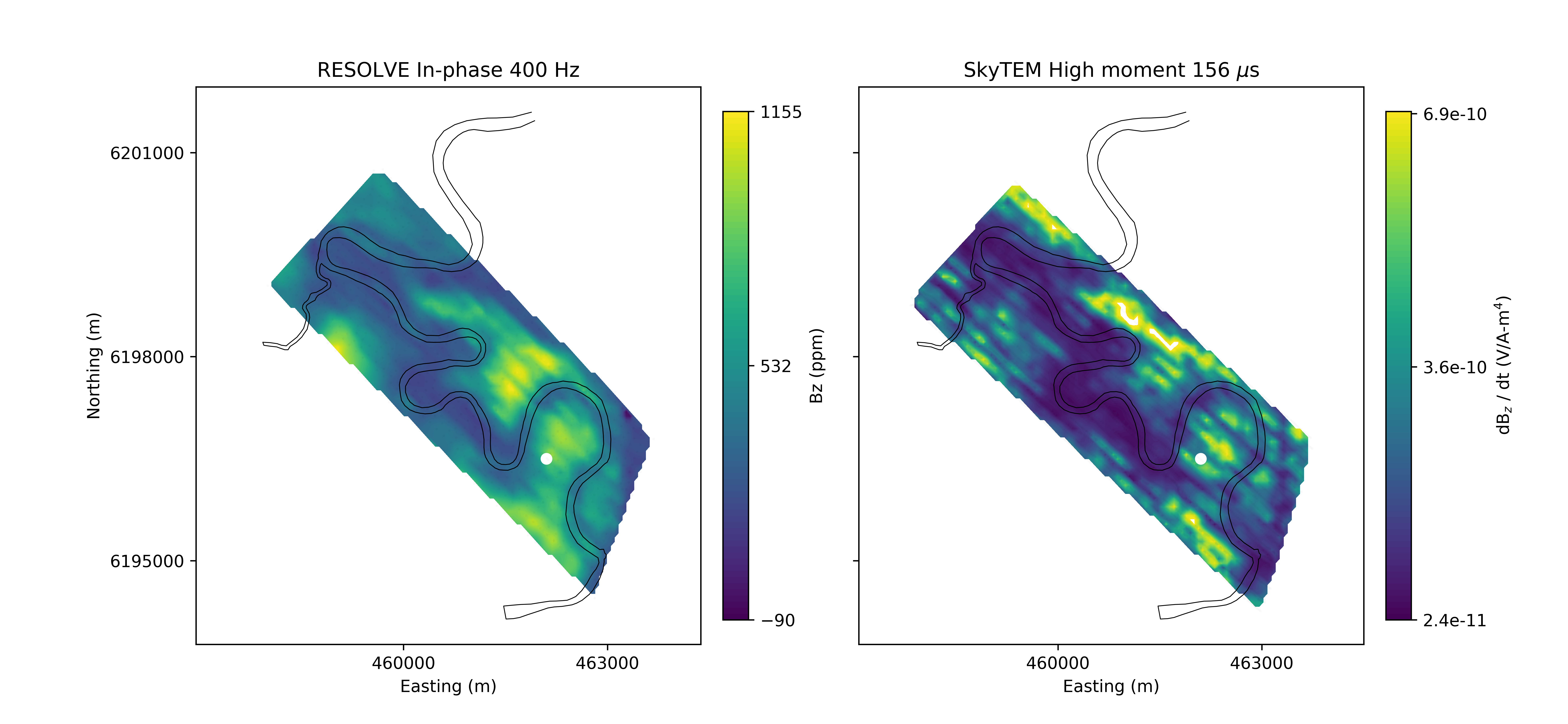
Figure 8:400 Hz In-phase RESOLVE data at (left) and High Moment SkyTEM data at 156 μ s. The white dot at (462100m, 6196500m) on both images is the location of the stations chosen to demonstrate the 1D inversions in frequency and time.
5.2.11D Inversion of RESOLVE and SkyTEM soundings
We have selected a sounding location (462100m, 6196500m) at which to perform 1D inversions of the RESOLVE and SkyTEM (High Moment) data. The observed data at this location are shown in Figure 9 (b) and (c). For the RESOLVE inversion, we consider the horizontal co-planar data collected at 400 Hz, 1800 Hz, 8200 Hz, 40 000 Hz, and 130 000 Hz. For the noise model, we assign 10% error for the three lowest frequencies and 15% error for the two highest; a noise floor of 20ppm is assigned to all data. The inversion mesh uses cells that expand logarithmically with depth, starting at the surface with a finest cell size of 1m. The forward simulation is carried out on the cylindrically symmetric mesh, similar to the previous example. In the inversion, we employ a Tikhonov regularization in which length scales have been omitted in the regularization function. A fixed trade-off parameter of is used, is set to be 1, and is . A half-space reference model with conductivity 0.1 S/m is used, this also served as the starting model for the inversion. The inversion reached target misfit after 2 iterations. The resulting model and data fits are shown in Figure 9. Very close to the surface, we recover a resistor, while below that, we recover a conductive unit (2 S/m). Examining the data (Figure 9b), we see that the real components are larger in magnitude than the imaginary, and that with increasing frequency, the magnitude of the imaginary component decreases while the real component increases; such behaviour is consistent with an inductive- limit response, and we thus expect to recover conductive structures in the model.
For the time domain inversion, we consider the SkyTEM high moment data. We use the source waveform shown in the inset plot in Figure 9 (c). For data, we use 21 time channels from 47 μs to 4.4 ms; the latest three time channels (5.6ms, 7ms and 8.8 ms) are not included. For data errors, we assign a 12% uncertainty and a floor of V/Am4. We again use a Tikhonov regularization, here with and . The trade-off parameter is . A half-space starting model of 0.1 S/m is again employed. For the reference model, we use the model recovered from the RESOLVE 1D inversion. As we are using the high-moment data, we do not expect the SkyTEM data to be as sensitive to the near surface structures as the RESOLVE data. By using the model recovered in the RESOLVE inversion as the starting model for the SkyTEM inversion, we can assess agreement between the two and isolate structures that are introduced by the SkyTEM inversion. The inversion reached the target misfit after 3 iteration and the results are shown in Figure 9. At this location, there is good agreement in the models recovered from the RESOLVE and SkyTEM data, with both supporting a near-surface resistor and showing a deeper conductive structure.
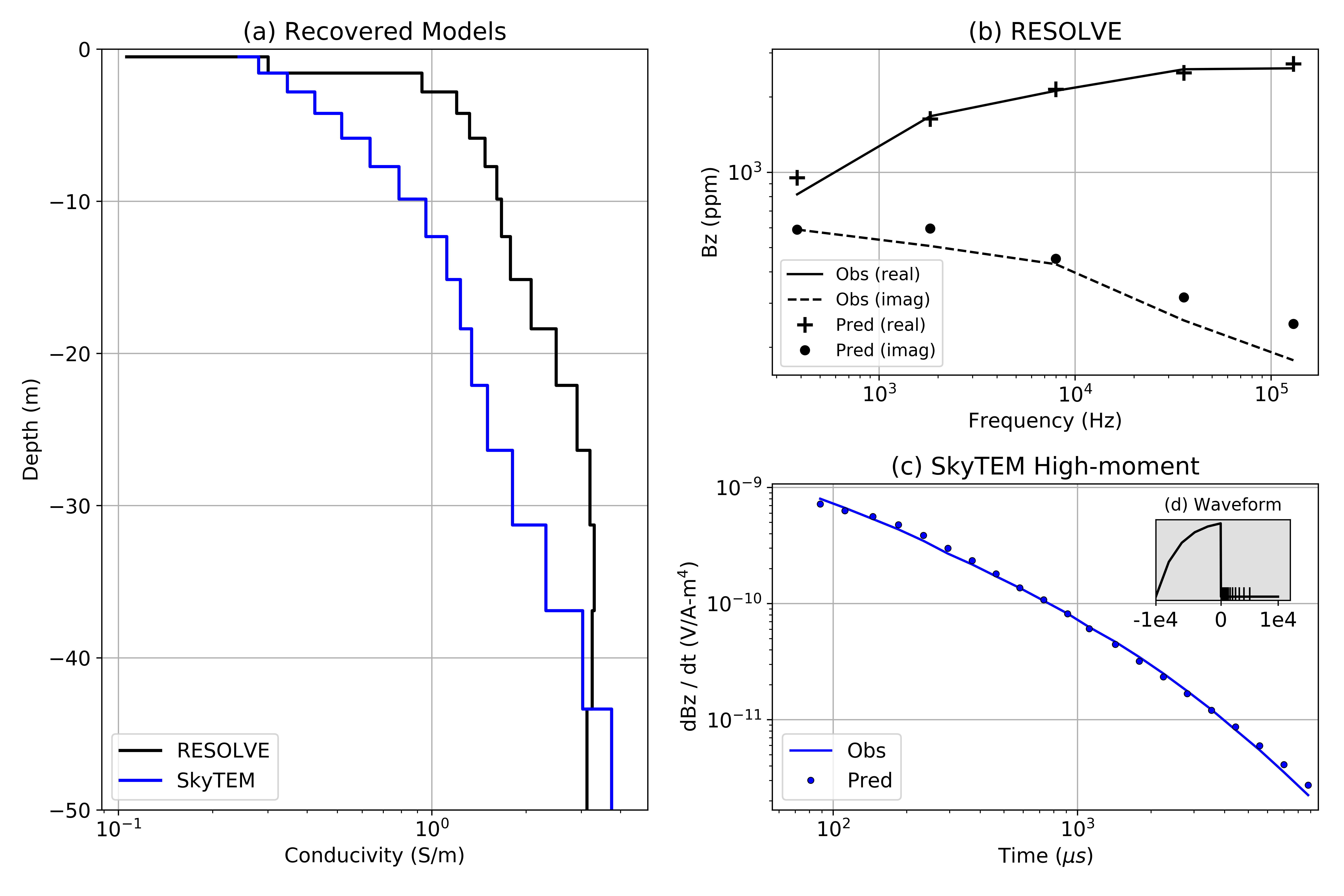
Figure 9:(a) Models recovered from from the 1D inversion of RESOLVE (back) and SkyTEM (blue) data at the location (462100m, 6196500m). (b) Observed (lines) and predicted (points) frequency domain data. (c) Observed and predicted time domain data. (d) Source waveform used in for the SkyTEM inversion, the x-axis is time (μ s) on a linear scale.
5.2.2Stitched 1D inversion of RESOLVE data
Next, we perform a stitched 1D inversion of the RESOLVE data set. With this example, we aim to demonstrate a practical inversion workflow that will run on modest computational resources. As such, we have heavily downsampled the data set, taking 1021 stations of the 40 825 collected. A 1D stitched inversion is a relatively straight-forward approach for creating a conductivity model - each sounding is inverted independently and the inversion results are then assembled to create a 3D model. This can be a valuable quality-control step prior to adopting more advanced techniques such as including lateral or 3D regularization across soundings or even performing a 3D inversion. In cases where the geology is relatively simple, a stitched 1D inversion may be sufficient. The inversion parameters are the same as those used in the inversion of the RESOLVE sounding discussed in the previous section. A plan- view of the recovered model 9.9m below the surface is shown in Figure 10a. A global χ - factor of 0.74 was reached, and plots comparing the real component of the observed and predicted data at 400Hz are shown in Figures 10 (b) & (c).
The recovered model (Figure 10a), bears similar features to the models found by Viezzoli et al. (2010) (Figure 4 of Viezzoli et al. (2010)) and by Yang (2017). In general, the northwestern portion of the Murray river is more resistive, in particular near (459 000m, 6 200 000m) and (460 000m, 6 198 000m) while the southeastern portion of the river is more conductive. Two mechanisms of river salinization have been discussed in Munday et al. (2006)Viezzoli et al. (2010): the resistive regions are attributed to a “losing” groundwater system, in which freshwater from the Murray River discharges to adjacent banks, while the conductive regions are attributed to a “gaining” system, in which regional saline groundwater seeps into the river.

Figure 10:(a) Conductivity model 9.9m below the surface from a stitched 1D inversion of RESOLVE data. (b) Real component of the observed RESOLVE data at 400Hz. (c) Real component of the predicted data at 400Hz.
5.3Steel-Cased Well: Sensitivity Analysis for a Parametric Model
The purpose of this example is to demonstrate the modular implementation of simpegEM and how it can be used to experiment with simulation and inversion approaches. Conducting electromagnetic surveys in settings where steel casing is present is growing in interest for applications such as monitoring hydraulic fracturing or enhanced oil recovery Hoversten et al., 2015Um et al., 2015Commer et al., 2015Hoversten et al., 2014Marsala et al., 2015Cuevas, 2014Weiss et al., 2015Yang et al., 2016. Steel is highly conductive (), has a significant magnetic permeability () Wu & Habashy, 1994. This is a large contrast to typical geologic settings, with conductivities typically less than 1 S/m and permeabilities similar to that of free space, . In addition to the large physical property contrast, the geometry of well casing also presents a significant computational challenge. Well casing is cylindrical in shape and only millimeters thick, while the geologic structures we aim to characterize are on the scale of hundreds of meters to kilometers. Inverting electromagnetic data from such settings requires that we have the ability to accurately simulate and compute sensitivities for models with casing and 3D geologic variations. One strategy that may be considered is using a primary- secondary approach, simulating the casing in a simple background and using these fields to construct a source for the secondary problem which considers the 3 dimensional structures of interest Heagy et al., 2015. Here, we demonstrate how the framework can be employed to implement this approach and compute the sensitivities. The parametric representation of the model allows us to investigate the expected data sensitivity to specific features of the model such as the location, spatial extent and physical properties of a geologic target. Such an analysis may be used to investigate how well we expect certain features of the model to be resolved in an inversion and it could be employed as a survey design tool. In what follows, we outline the general approach and then discuss a specific implementation. The script used to generate this example is available at: https://doi.org/10.6084/m9.figshare.5036123.
5.3.1Approach
In this example we design a survey to resolve a conductive body in a reservoir layer in the presence of a vertical, steel-cased well as shown in Figure 11. To calculate the sensitivity of the data with respect to each model parameter requires that we be able to simulate and calculate derivatives of each component used to simulate data.
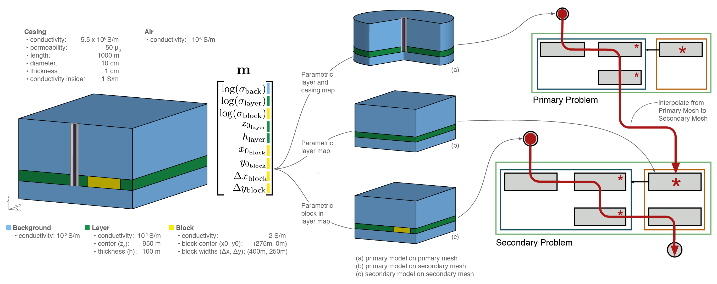
Figure 11:Setup of parametric models and calculation of the sensitivity for a primary secondary approach of simulating 3D geology and steel casing.
We use a primary-secondary approach, as described in Heagy et al. (2015). The physical properties, fields and fluxes are composed of two parts, a primary and a secondary part. For example in the E-B formulation, , , , . A primary problem, which includes the cylindrically symmetric part of the model (casing, source, and layered background) is defined
This primary problem is solved on a cylindrically symmetric mesh with cells fine enough to capture the width of the casing and its solution yields the primary fields. The primary fields are then interpolated to a 3D tensor mesh, suitable for discretizing 3D reservoir-scale features. The primary fields are used to construct the source current density for the secondary problem, given by
By solving the secondary problem, we then obtain secondary fields and fluxes. These are sampled by the receivers to create predicted data.
In equation 25, we see that the source term, has model dependence through σ, and . Typically primary-secondary approaches are used when the background is assumed to be known, as it is captured in the primary. Here, however, we do not wish to assume that the background is known; in practice it may be constrained, but it is not generally well known. The primary solution is used instead to separate the contributions of the casing and the block so that we can avoid a potentially crippling assumption. This approach allows an appropriately tailored mesh to be constructed for each problem. Thus, we require derivatives not only on the 3D secondary mesh, but also derivatives of the primary fields (in this case on a cylindrically symmetric mesh). To implement this type of primary-secondary problem, we construct a Primary-Secondary source which solves the primary problem to provide the primary fields. Since all derivatives are implemented for the primary problem, when computing sensitivities for the secondary problem, the derivatives due to the primary problem are accounted for in the contributions of the source term to the derivative. This is conceptually shown in Figure 11.
For this example, we wish to investigate how sensitive the specified survey is to aspects of the model which we might want to resolve in a field survey, such as the geometry and location of the anomalous body, as well as the physical properties of the geologic units. A voxel-based description of the model does not promote investigation of these questions, so we will instead apply a parametric description of the model. The model is parameterized into nine parameters which we consider to be unknowns (, , , , , , , , ). In what follows, we examine the sensitivity of the data with respect to these model parameters.
5.3.2Implementation
The model we use is shown in Figure 11. It consists of a 1km long vertical steel cased well (diameter: 10 cm, thickness: 1cm) with conductivity S/m, and magnetic permeability . The casing is assumed to be filled with fluid having a conductivity of 1S/m. The background has a resistivity of , and the 100m thick reservoir layer has a resistivity of . The target of this survey is the conductive block (2S/m) with dimensions . The source used consists of two grounded electrodes, a positive electrode coupled to the casing at a depth of 950m, and a return electrode 10km from the wellhead on the surface. We consider a frequency-domain experiment at a transmitting frequency of 0.5Hz and 1A current. For data, we consider two horizontal components ( and ) of the real part of the electric field measured at the surface.
To accomplish this simulation and sensitivity calculation, we construct 3 mappings, shown conceptually in Figure 11, in order to obtain: (1) on the primary (cylindrical) mesh, (2) on the secondary mesh (as is needed in equation 25) and (3) σ on the secondary mesh. Differentiability of the electrical conductivity models with respect to each of the 9 parameters is achieved by constructing the model using arctangent functions (cf. Aghasi et al. (2011)McMillan et al. (2015)). Each of these parameterizations can be independently tested for second-order convergence to check the validity of the computation of the derivatives (cf. Haber (2014)).
The source term for the secondary fields requires that we simulate the primary fields. For this, we use the mapping of to on the primary mesh and employ the H-J formulation of Maxwell’s equations in the frequency domain in order to describe a vertically and radially oriented current density and a rotational magnetic field. In this simulation, we also consider the permeability of the casing. The source consists of a wire-path terminating downhole at -950m where it is coupled to the casing. At the surface, the return electrode is 10km radially away from the well[3]. With these parameters defined, we have sufficient information to solve the primary problem and thereby obtain the primary electric field everywhere in the simulation domain. The real, primary current density for this example is shown in Figure 12.
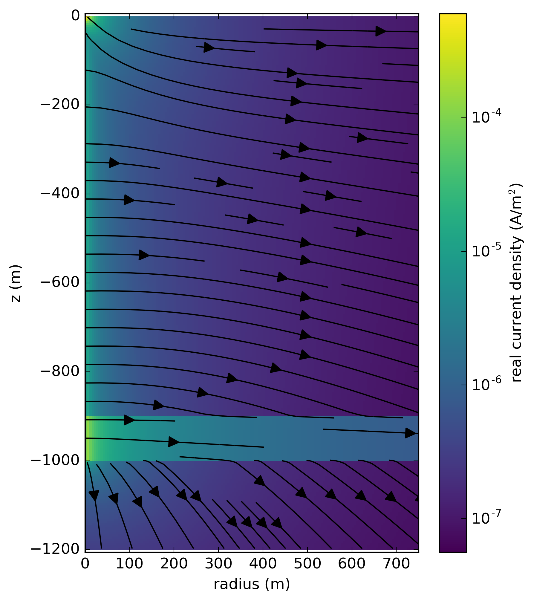
Figure 12:Cross sectional slice of primary (casing + background) real current density. The colorbar is logarithmically scaled and shows the amplitude of the real current density.
This primary field is described on the cylindrical mesh, so in order to use it to construct the source term for the secondary problem, we interpolate it to the 3D tensor mesh. The remaining pieces necessary for the definition of the secondary source on the 3D mesh are defining σ and ; this is achieved through the mappings defined above. The primary problem and source, along with the mapping required to define , are used to define a primary-secondary source, which solves a forward simulation to compute the secondary source-current, , shown in Figure 13. Note that the source current density is only present where there are structures in the secondary model that were not captured in the primary, in this case, where the conductive block is present.
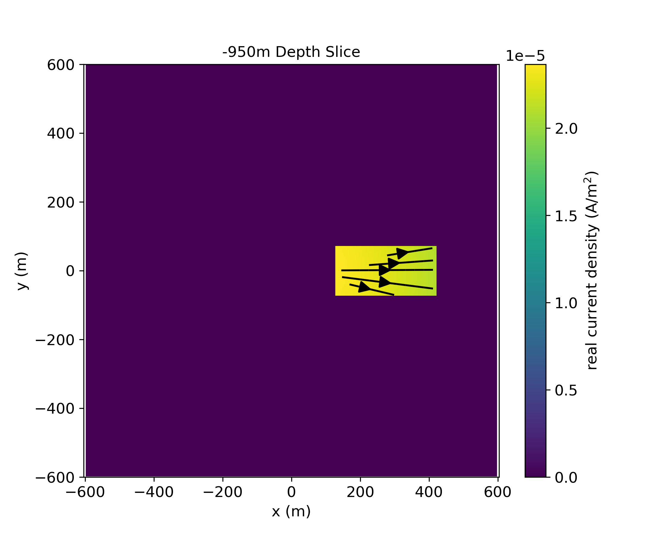
Figure 13:Depth slice at z=-950m showing the source current density for the secondary problem.
With the source term for the secondary problem defined, the secondary problem is then solved resulting in the predicted data at the surface. Here, we focus our attention to the real x, y components of the electric field, as shown in Figure 14. The top two panels show the total (casing and conductive target) x-component (a) and y-component (b) of the electric field while the bottom two panels show the secondary (due to the conductive target, outlined in white) x-component (c) and y-component (d) of the electric field. As expected, the total electric field is dominated by the source that is located in the casing. As shown in Figure 12 the majority of the current is exiting into the layer at depth, but current is still emanating along all depths of the casing. Measured electric fields at the surface are sensitive to the currents that come from the top part of the casing and hence the observed fields are strongest closest to the pipe and they fall off rapidly with distance. The behavior of the secondary electric field is, to first order, like that expected from a dipole at depth oriented in the x-direction. It has a broad smooth signature at the surface.
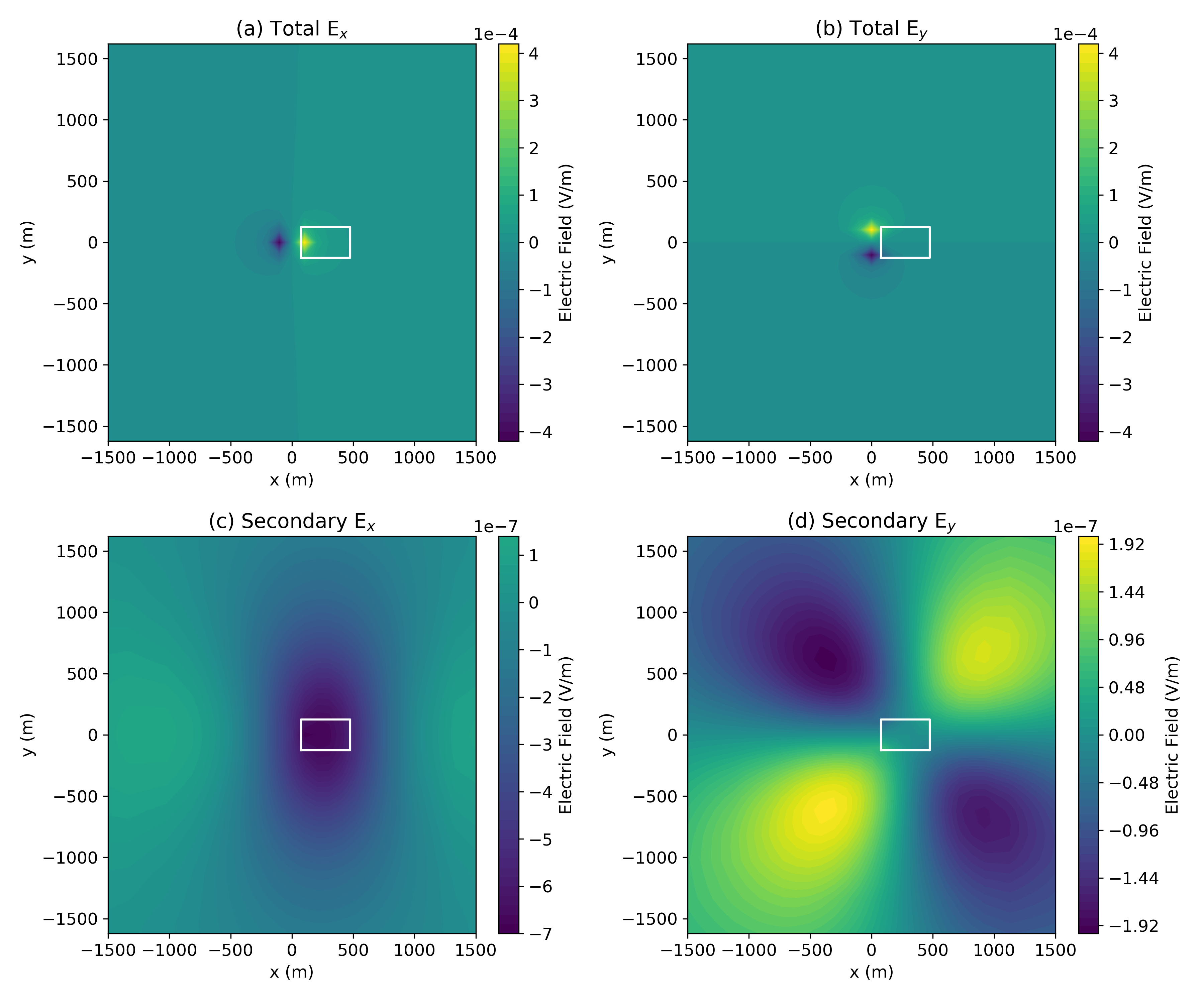
Figure 14:Simulated real electric field data as measured at the surface using a primary secondary approach for casing and a conductive target (outlined in white). The upper panels show the total (a) and (b); the lower panels show the secondary (due to the conductive block) (c) and (d). Note that the colorbars showing the secondary electric fields are not on the same scale. The limits of the colorbars have been set so that the zero-crossing is always shown in the same color.
Now that the pieces are in place to perform the forward simulation, we want to compute the sensitivity. Generally, we do not form the full sensitivity when performing an inversion as it is a large, dense matrix. Here however, since the inversion model is composed of only nine parameters, the final sensitivity matrix is small (nine by number of data). The steps followed to stitch together and compute the sensitivity are shown in the diagram in Figure 11. To check the simulation approach for this example, the sensitivity is tested for second-order convergence (cf. Haber (2014)).
Figures 15, 16 and 17 shows the sensitivity of both the real (left), and real (right) data with respect to each of the 9 model parameters. Note that the colorbars are not identical in each image and the units of the sensitivity are dependent on the parameter under consideration. In each image, the white outline shows the horizontal location of the block.
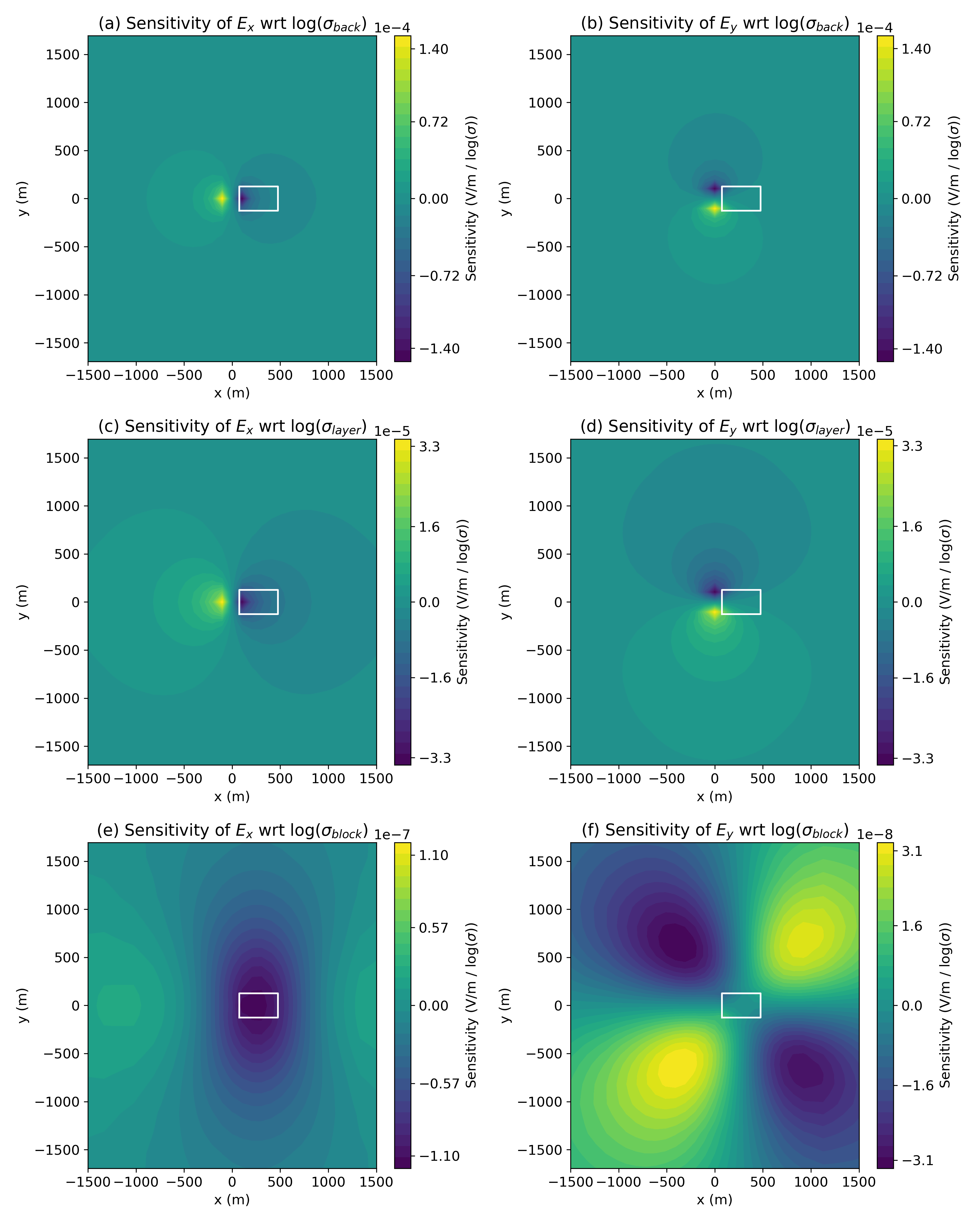
Figure 15:Sensitivity of surface real (left) and (right) data with respect to the physical properties, ()
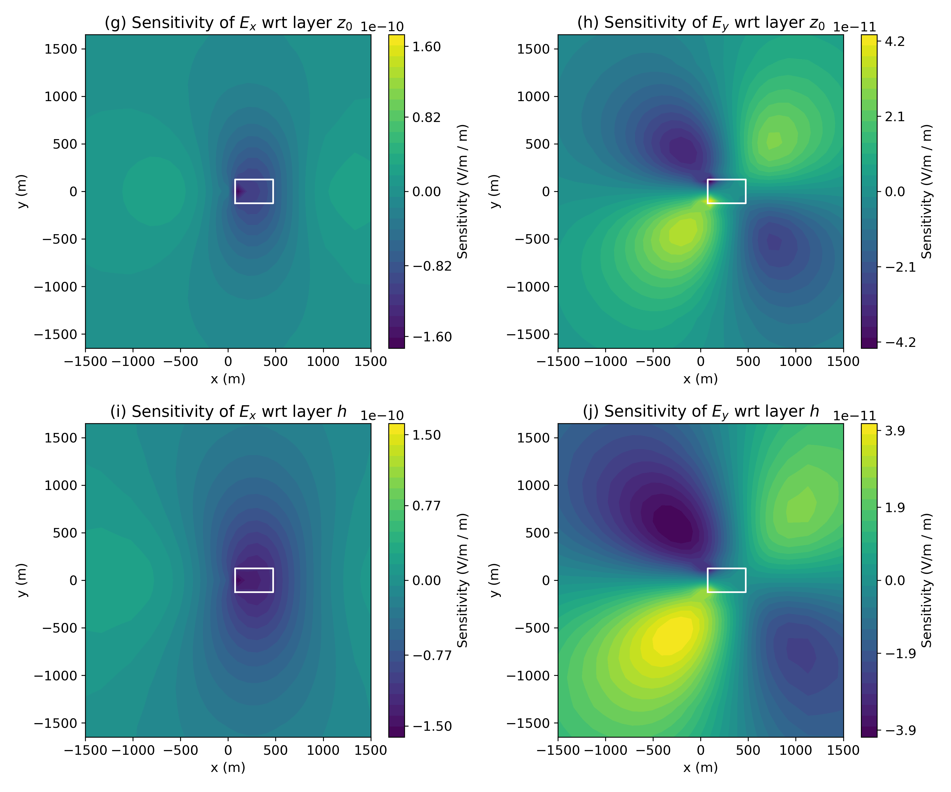
Figure 16:Sensitivity of surface real (left) and (right) data with respect to the layer geometry, ()
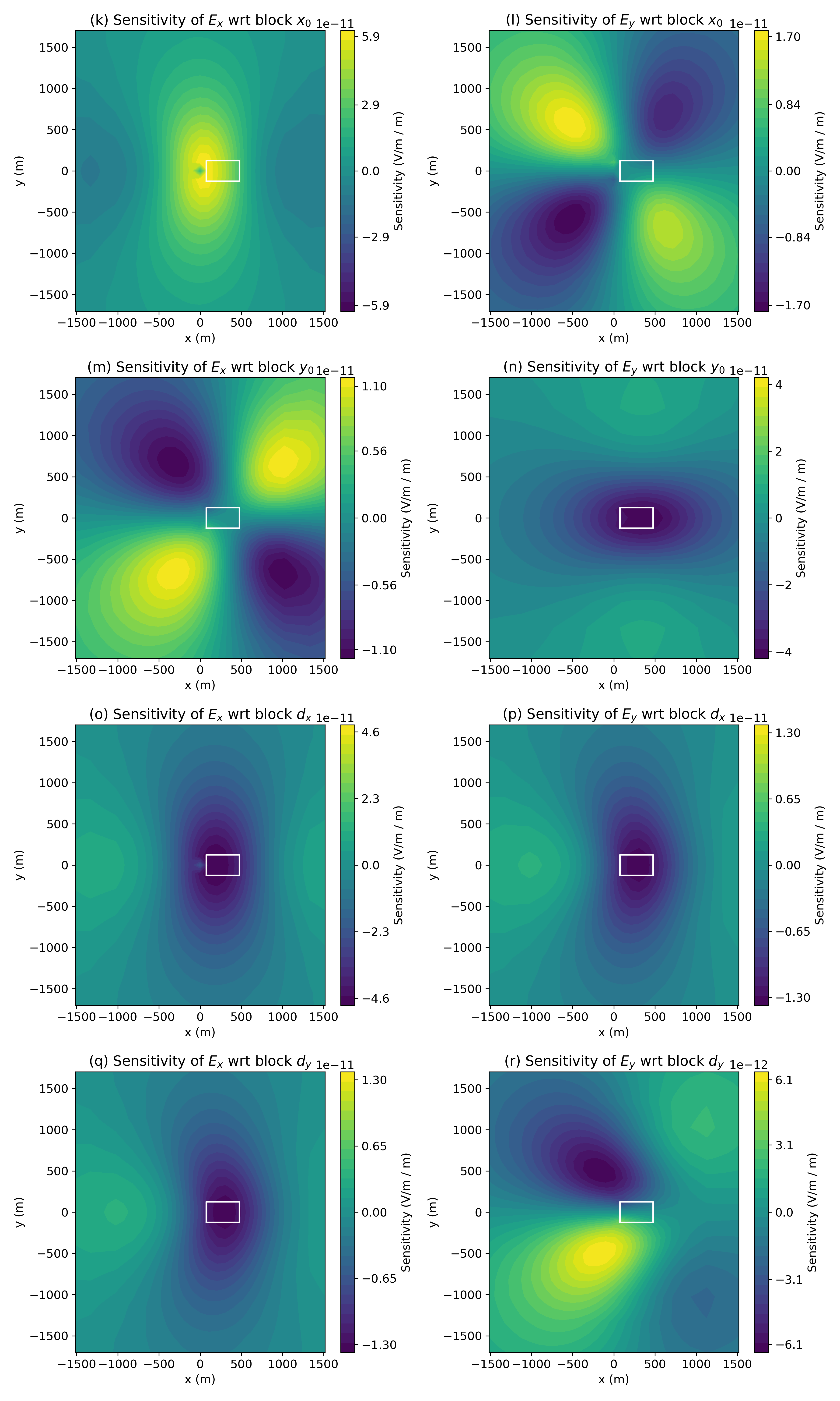
Figure 17:Sensitivity of surface real (left) and (right) data with respect to the block geometry, ()
In Figure 15, we focus on the physical properties of the background layer and block, all parametrized in terms of . Clearly, the conductivity of the background has the largest influence on the data, in particular near the well (at the origin), followed by the conductivity of the layer, where the injection electrode is situated. There are 4 orders of magnitude difference between the maximum sensitivity of the data with respect to the conductivity of the block and that of the background. This indicates that in order to resolve such an anomalous body, the background must be well-constrained. When looking at Figure 15 (f), we see that the areas of largest sensitivity of the data with respect to the physical properties of the block are spatially distant from the body and the well. This indicates that if one is designing a survey, it may be advantageous to collect data in these regions as these are also regions where the influence of the properties of the background are less dominant.
In Figure 16, we focus on the depth and thickness of the layer. Note that the depth and thickness of the block are constrained to be the same as the layer, so the character of the sensitivity is influenced by the presence of the block. Here, the units of the sensitivity are . Similarly, Figure 17 shows the sensitivity with respect to the geometric properties of the block.
To compare between the physical properties and geometry of the model, the scales of interest must be taken into consideration. In Table 1, we show the maximum amplitude of the sensitivity with respect to each individual model parameter. From this, we approximate the sensitivity as linear about the true model and compute the perturbation required to cause a change of in the data (). For ease of comparison, the perturbations in the log-conductivity of the background, layer, and block were converted to linear conductivity by
In table 1, we see that to cause a perturbation in the data by , requires a 0.007% change in the conductivity of the background, while the conductivity of the block would need to change by 0.8% to have a comparable impact in the data. In comparing between physical properties and geometric features of the model, we see that a change in the conductivity of the block by 0.8% has a similar impact in the data as moving of the block by . For a change in of the block to have a comparable impact in the data would require that it be perturbed by . However, the data are more sensitive to ; a perturbation of , about 1/3 of that required in the data, would result in a change in the measured responses.
Table 1:Comparison of the maximum amplitude of the sensitivity with respect to each model parameter, and the approximate perturbation in that parameter required to produce a change in the measured data. The conversion from a perturbation in log-conductivity to conductivity is given by equation 26. The perturbation in conductivity is also provided in terms of a percentage of the true model conductivity.
| parameter | Units of | max | perturbation required to | max | perturbation required to | ||
| Sensitivity, | wrt | cause in | wrt | cause in | |||
| 1.5e-04 | 6.6e-08 | (6.6e-04%) | 1.5e-04 | 6.6e-08 | (6.6e-04%) | ||
| 3.5e-05 | 2.9e-06 | (2.9e-03%) | 3.4e-05 | 2.9e-06 | (2.9e-03%) | ||
| 1.2e-07 | 1.7e-02 | (8.4e-01%) | 3.3e-08 | 6.1e-02 | (3.1e+00%) | ||
| 1.7e-10 | 5.8e+00 | 4.4e-11 | 2.3e+01 | ||||
| 1.6e-10 | 6.2e+00 | 4.1e-11 | 2.4e+01 | ||||
| 6.2e-11 | 1.6e+01 | 1.8e-11 | 5.6e+01 | ||||
| 1.2e-11 | 8.5e+01 | 4.2e-11 | 2.4e+01 | ||||
| 4.8e-11 | 2.1e+01 | 1.5e-11 | 6.6e+01 | ||||
| 1.4e-11 | 7.3e+01 | 6.5e-12 | 1.5e+02 | ||||
Examining the nature of the sensitivity with respect to parameters describing the target of interest provides insight both into how one might design a survey sensitive to the target, and how well we may be able to resolve various geometric features or physical properties in the model. For the example shown here, we see that it may be advantageous to collect data away from the well and hundreds of meters offset from the block. These are regions where both the and data have high sensitivity to features of the target and are distant from the steel-cased well, where we have the highest sensitivity to the background. Thus, data collected in these regions may improve our ability to resolve the target of interest. The parametric definition of the model provides a mechanism for examining how well we might expect to resolve various aspects of the target, such as its spatial extent. There are clearly further questions that may be investigated here, including exploring survey parameters such as the impact of varying the frequency on our ability to resolve the block, or performing the same analysis for a time-domain survey. A modular framework, with accessible derivatives, is an asset for exploring these types of questions.
6Conclusion
The framework we have laid out has rigorously separated out various contributions to the electromagnetic equations in both time and frequency domain. We have organized these ideas into an object oriented hierarchy that is consistent across formulations and attends to implementation details and derivatives in a modular way. The organization of the EM framework and numerical implementation are designed to reflect the math. The goal is to create composable pieces such that electromagnetic geophysical inversions and forward simulations can be explored and experimented with by researchers in a combinatorial, testable manner.
We strive to follow best practices in terms of software development including version control, documentation unit testing, and continuous integration. This work and the SimPEG project are open-source and licensed under the permissive MIT license. We believe these practices promote transparency and reproducibility and we hope that these promote the utility of this work to the wider geophysics community.
Acknowledgments
The authors thank Dr. Eldad Haber for his invaluable guidance in the development and implementation of the framework. We also thank the growing community of SimPEG developers, in particular: Dr. Dave Marchant, Dr. Brendan Smithyman, Michael Mitchell, Thibaut Astic, Dominique Fournier, and Joseph Capriotti, have contributed to the SimPEG code-base; we are grateful for your contributions both to the code and the discussions in the development of SimPEG.
Thanks also to CSIRO for making the Bookpurnong data available and to Dikun Yang for conversations on the inversion of those data, and finally to the three anonymous reviewers whose comments improved the quality of the paper.
The funding for this work is provided through the Vanier Canada Graduate Scholarships Program.
Copyright © 2017 Heagy et al.
In most geophysical electromagnetic surveys, low frequencies or late-time measurements are employed. In these scenarios (eg. conductivities are typically less than 1S/m, and frequencies considered are generally less than 105 Hz), so displacement current can safely be ignored.
We use the term inversion model to describe a parameterized representation of the earth (e.g. voxel-based or parametric), even if the model is solely used for forward modelling, its form sets the context for the inverse problem and the parameter-space that is to be explored.
Due to the symmetry employed, the return electrode is a disc. Numerical experiments over a half-space show that the real, radial electric field from the cylindrical simulation exhibits the same character as the 3D simulation but is slightly reduced in magnitude.
- EM
- electromagnetics
- Yee, K. (1966). Numerical solution of initial boundary value problems involving maxwell’s equations in isotropic media. IEEE Transactions on Antennas and Propagation, 14(3), 302–307. 10.1109/TAP.1966.1138693
- Newman, G. A., & Alumbaugh, D. L. (1999). 20. Electromagnetic Modeling and Inversion on Massively Parallel Computers. In Three-Dimensional Electromagnetics (pp. 299–321). Society of Exploration Geophysicists. 10.1190/1.9781560802154.ch20
- Haber, E. (2014). Computational Methods in Geophysical Electromagnetics. Society for Industrial. 10.1137/1.9781611973808
- Haber, E., & Ascher, U. M. (2001). Fast Finite Volume Simulation of 3D Electromagnetic Problems With Highly Discontinuous Coefficients ∗. 22(6), 1943–1961.
- Li, Y., & Key, K. (2007). 2D marine controlled-source electromagnetic modeling: Part 1 — An adaptive finite-element algorithm. GEOPHYSICS, 72(2), WA51–WA62. 10.1190/1.2432262
- Kelbert, A., Meqbel, N., Egbert, G. D., & Tandon, K. (2014). ModEM: A modular system for inversion of electromagnetic geophysical data. Computers and Geosciences, 66, 40–53. 10.1016/j.cageo.2014.01.010
- Yang, D., Oldenburg, D. W., & Haber, E. (2014). 3-D inversion of airborne electromagnetic data parallelized and accelerated by local mesh and adaptive soundings. Geophysical Journal International, 196(3), 1492–1507. 10.1093/gji/ggt465
- Tikhonov, A. N., & Arsenin, V. Y. (1977). Solutions of Ill-Posed Problems. SIAM Review, 32, 1320–1322. http://www.getcited.org/pub/101760676
- Parker, R. L. (1980). The inverse problem of electromagnetic induction: Existence and construction of solutions based on incomplete data. Journal of Geophysical Research: Solid Earth, 85(B8), 4421–4428. 10.1029/JB085iB08p04421
- Constable, S. C., Parker, R. L., & Constable, C. G. (1987). Models From Electromagnetic Sounding Data. Geophysics, 52(3), 289–300.
- Oldenburg, D. D. W., & Li, Y. (2005). Inversion for applied geophysics: A tutorial. Investigations in Geophysics, 13, 1–85. 10.1190/1.9781560801719
- Pidlisecky, A., Singha, K., & Day-Lewis, F. D. (2011). A distribution-based parametrization for improved tomographic imaging of solute plumes. Geophysical Journal International, 187(1), 214–224. 10.1111/j.1365-246X.2011.05131.x
- McMillan, M. S., Oldenburg, D. W., Haber, E., & Christoph. (2015). Parametric 3D inversion of airborne time domain electromagnetics. 24th International Geophysical Conference and Exhibition, 1–5. 10.1071/ASEG2015ab101
- Kang, S., Cockett, R., Heagy, L. J., Oldenburg, D. W., & Facility, G. I. (2015). Moving between dimensions in electromagnetic inversions. 2, 5000–5004.
- Haber, E., & Oldenburg, D. (1998). Joint Inversion: A Structural Approach. Unknown, 63.
